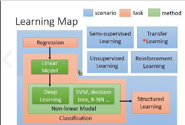
Learning Map

Regression: Case Study

$y = b + w\cdot{x_{cp}}$

$(x_{feature},\hat{y})$

Loss function L

input: a function output: how bad it is

$L(f)=L(w,b)=\displaystyle\sum_n(\hat{y}^n-(b+w\cdot{x_{feature}^n}))^2$

Pick the "Best" Function

$f^*=arg \displaystyle\min_fL(f)$

$w^*,b^*=arg\displaystyle\min_{w,b}L(w,b)=arg\displaystyle\min_{w,b}\displaystyle\sum_n(\hat{y}^n-(b+w\cdot{x_{feature}^n}))^2$

Gradient Descent

• Consider loss function L(w) with two parameter w, b:
• • (Randomly) Pick an initial value $w^0,b^0$
  • Compute $\frac{\partial{L}}{\partial{w}}|w=w^0,b=b^0,\frac{\partial{L}}{\partial{b}}|w=w^0,b=b^0$
  • $w^1\gets{w^0-\eta\frac{\partial{L}}{\partial{w}}|w=w^0},\qquad b^1\gets{b^0-\eta\frac{\partial{L}}{\partial{w}}|w=w^0,b=b^0}$ $\eta$:"learning rate"
  • ... Many iteration

Local optimal, not global optimal...

In linear regression, the loss function L is convex, so no local optimal

$L(w,b)=\displaystyle\sum_n(\hat{y}^n-(b+w\cdot{x_{feature}^n}))^2$

$\frac{\partial{L}}{\partial{w}}=\displaystyle\sum_n{2(\hat{y}^n-(b+w\cdot{x_{feature}^n}))(-x_{feature}^n)}$

$\frac{\partial{L}}{\partial{b}}=\displaystyle\sum_n{2(\hat{y}^n-(b+w\cdot{x_{feature}^n}))(-1)}$

Regularization

$L=\displaystyle\sum_n{(\hat{y}^n-(b+\sum{w_ix_i}))^2}+\lambda\sum{(w_i)^2}$

The functions with smaller $w_i$ are better

Training error: larger$\lambda$, considering the training error less

We prefer smooth function, but don't be too smooth

Gradient Descent

$\theta^*=arg\displaystyle\min_{\theta}{L(\theta)}$ L: loss function $\theta$: parameters

Suppose that $\theta$ has two variables $\{\theta_1, \theta_2\}$

Randomly start at $\theta^0=\begin{bmatrix}\theta_1^0\\ \theta_2^0\end{bmatrix}$

$\begin{bmatrix}\theta_{1}^1\\ \theta_2^1\end{bmatrix}=\begin{bmatrix}\theta_1^0\\ \theta_2^0\end{bmatrix} - \eta \begin{bmatrix} \partial{L(\theta_1^0)}/\partial{\theta_1}\\ \ \partial{L(\theta_2^0})/ \partial{\theta_2}\end{bmatrix}\qquad \nabla L(\theta)=\begin{bmatrix} \partial{L(\theta_1)}/\partial{\theta_1}\\ \ \partial{L(\theta_2})/ \partial{\theta_2}\end{bmatrix}$

...

$\theta^i=\theta^{i-1}-\eta\nabla L(\theta^{i-1})$

Watch picture

• Popular & Simple Idea: Reduce the learning rate by some factor every few epochs
• E.g. 1/t decay: $\eta^t = \eta/\sqrt{t+1}$

Adagrad

Divide the learning rate of each parameter by the root mean square of its previous derivatives

$w^{t+1}\gets{w^t-\frac{\eta^t}{\sigma^t}}g^t$

$\eta^t=\frac{\eta}{\sqrt{t+1}}\qquad g^t=\frac{\partial{C(\theta^t)}}{\partial{w}} \qquad \sigma^t$: root mean square of the previous derivatives of parameter w

$w^1\gets{w^0-\frac{\eta^0}{\sigma^0}g^0}\qquad \sigma^0=\sqrt{(g^0)^2}$

$w^2\gets{w^1-\frac{\eta^1}{\sigma^1}g^1}\qquad \sigma^1=\sqrt{\frac{1}{2}[(g^0)^2+(g^1)^2]}$

...

$w^{t+1}\gets{w^t-\frac{\eta^t}{\sigma^t}g^t}\qquad \sigma^t=\sqrt{\frac{1}{t+1}\displaystyle\sum_{t=0}^t{(g_i)^2}}$

$\therefore w^{t+1}\gets{w^t-\frac{\eta}{\sqrt{\sum_{i=0}^t{(g^i)^2}}}g^t}$

best step: $\frac{|First-derivative|}{Second-derivative}$

Stochastic Gradient Descent

faster

Pick an example $x^n$

$L^n = (\hat{y}^n-(b+\sum{w_ix_i^n}))^2$ Loss for only one example

$\theta^i=\theta^{i-1}-\eta\nabla L^n(\theta^{i-1})$

Feature Scaling

make different features have the same scaling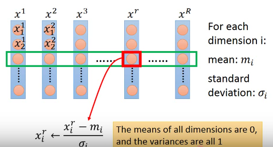

More limitation

local minima

stuck at saddle point

very slow at the plateau

Where does the error come from?

error due to "bias"

error due to "variance"

$f^*$ is an estimator of $\hat{f}$

简单model，small variance Simple model is less influenced by the sampled data.

Bias: If we average all the $f^*$, it is close to $\hat{f}$

简单model，large bias

Large bias?

Redesign your model:

• Add more features as input
• A more complex model

Large variance

• More data
• Regularization

Cross Validation

N-fold Cross Validation

Classification: Probabilistic Generative Model

$P(C_1|x)=\frac{P(x|C_1)P(C_1)}{P(x|C_1)P(C_1)+P(x|C_2)P(C_2)}$

Generative Model $P(x)=P(x|C_1)P(C_1)+P(x|C_2)P(C_2)$

Gaussian Distribution

$f_{\mu,\Sigma}(x)=\frac{1}{(2\pi)^{D/2}}\frac{1}{|\Sigma|^{1/2}}exp\{-\frac{1}{2}(x-\mu)^T\Sigma^{-1}(x-\mu)\}$

$P(x|c_n)=f_{\mu^n,\Sigma^n}(x)$

Input: vector x, output: probability of sampling x

The shape of the function determines by mean $\mu$ and convariance matrix $\Sigma$

Maximum Likelihood

We have n examples: $x^1, x^2, \cdots, x^n$, feature m 个

$L(\mu, \Sigma) = \displaystyle\prod_n{f_{\mu,\Sigma}(x^n)}$

$\mu^*,\Sigma^*=arg\displaystyle\max_{\mu,\Sigma}L(\mu,\Sigma)$

$\mu^*=\frac{1}{n}\displaystyle\sum_n{x^n}$ (average) 会得到一个$m\times{1}$的矩阵$\Sigma^*=\frac{1}{n}\displaystyle\sum_n{(x^n-\mu^*)(x^n-\mu^*)^T}$ $m\times{m}$的矩阵

Modifying Model

假设两个classification共享 the same convariance matrix $\Sigma$

Class 1: 79个， Class 2: 61个

Find $\mu^1,\mu^2,\Sigma$ maximizing the likelihood $L(\mu^1,\mu^2,\Sigma)$

$L(\mu^1,\mu^2,\Sigma)=\displaystyle\prod_{n_1}{f_{\mu^1,\Sigma}}(n_1)\times{\displaystyle\prod_{n_2}{f_{\mu^2,\Sigma}}(n_2)}$

$\mu^1$ and $\mu^2$ is the same $\Sigma=\frac{79}{140}\Sigma^1+\frac{61}{140}\Sigma^2$

变成linear model

Probability Distribution

Posterior Probability

$\begin{matrix} P(C_1|x)=\frac{P(x|C_1)P(C_1)}{P(x|C_1)P(C_1)+P(x|C_2)P(C_2)} \\ = \frac{1}{1+\frac{P(x|C_2)P(C_2)}{P(x|C_1)P(C_1)}} = \frac{1}{1+exp(-z)}=\sigma(z) \\ z = \ln{\frac{P(x|C_1)P(C_1)}{P(x|C_2)P(C_2)}} \end{matrix}$

$\sigma(z)$: sigmoid function

经过运算，

$\begin{matrix} z=\ln{\frac{|\Sigma^2|^{1/2}}{|\Sigma^1|^{1/2}}}-\frac{1}{2}x^T(\Sigma^1)^{-1}x +(\mu^1)^T(\Sigma^1)^{-1}x-\frac{1}{2}(\mu^1)^T(\Sigma^1)^{-1}\mu^1 \\ +\frac{1}{2}x^T(\Sigma^2)^{-1}x-(\mu^2)^T(\Sigma^2)^{-1}x+\frac{1}{2}(\mu^2)^T(\Sigma^2)^{-1}\mu^2+\ln{\frac{N_1}{N_2}} \end{matrix}$

$\Sigma_1=\Sigma_2=\Sigma$

$\begin{matrix} z=(\mu^1-\mu^2)^T\Sigma^{-1}x-\frac{1}{2}(\mu^1)^T\Sigma^{-1}\mu^1+\frac{1}{2}(\mu^2)^T\Sigma^{-1}\mu^2+\ln{\frac{N_1}{N_2}} \\ =w^Tx+b \end{matrix}$

$P(C_1|x)=\sigma(w\cdot{x}+b)$

Logistic Regression

$f_{w,b}(x)=\sigma(\displaystyle\sum_i{w_ix_i+b)}$

Training data: $(x^n,\hat{y}^n)$

$\hat{y}^n$: 1 for class 1, 0 for class 2

$L(f)=\displaystyle\sum_nC(f(x^n),\hat{y}^n)$

Cross entropy:

$C(f(x^n),\hat{y}^n)=-[\hat{y}^n\ln{f(x^n)}+(1-\hat{y}^n)\ln{(1-f(x^n))}]$

partial it,

$w_i\gets{w_i-\eta\displaystyle\sum_n-(\hat{y}^n-f_{w,b}(x^n))x_i^n}$

Just the same as linear regression

Discriminative v.s Generative

discriminative: logistic

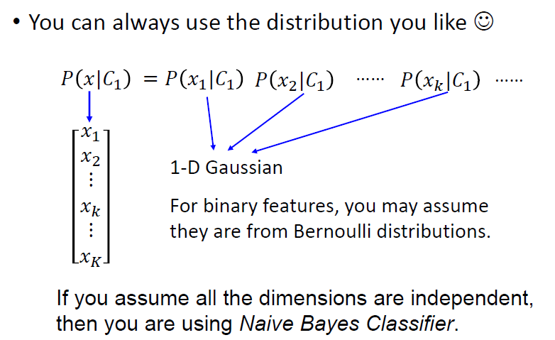
generative: naive

结果是不一样的

discriminative 效果比 generative 好

Benefit of generative model

在数据量比较小的时候，generative会赢

noisy, gen wins

priors and class-dependent probabilities can be estimated from different sources.

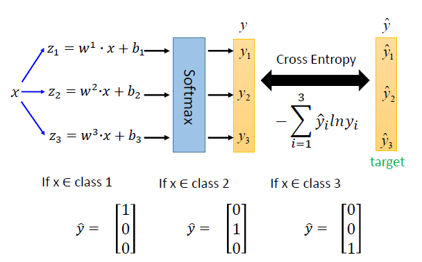
Multi-class Classification

$\begin{matrix} C_1:w^1\cdot{x}+b_1\qquad z_1= w^1\cdot{x}+b_1 \\ C_2:w^2\cdot{x}+b_2\qquad z_2= w^2\cdot{x}+b_2 \\ C_3:w^3\cdot{x}+b_3 \qquad z_3= w^3\cdot{x}+b_3 \end{matrix}$$x = y$

$\begin{matrix} y_1=e^{z_1}/\displaystyle\sum_{j=1}^3{e^{z_j}} \\ y_2=e^{z_2}/\displaystyle\sum_{j=1}^3{e^{z_j}} \\ y_3=e^{z_3}/\displaystyle\sum_{j=1}^3{e^{z_j}} \end{matrix} \qquad Softmax$

$y_i=P(C_i|x)$

上图有误：

cross entropy: $-\displaystyle\sum_{i=1}^3{\hat{y_i}\ln{y_i}}$

Limitation of Logistic Regression

非线性

Brief Introduction of Deep Learning

deep = Many hidden layers

Matrix Operation

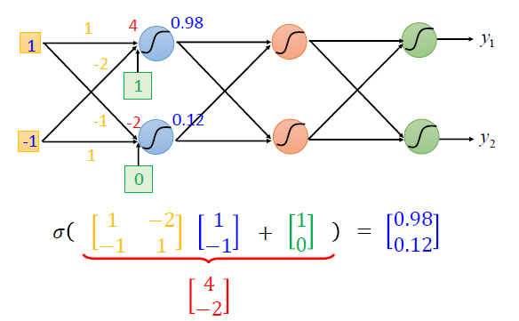
$\sigma(w^La^{L-1}+b^L)$

$y=f(x)=\sigma(w^L\cdots{\sigma(w^2\sigma(w^1x+b^1)}+b^2)+\cdots+b^L)$

Backprogation

To compute the gradients effiently, we use backpropagation